Predicting and designing proteins (1): How protein structure became a computational problem

12 Jul, 2026

Recently I’ve been working on predictive and generative models of proteins. Quite a shift in expertise, if you ask me! Therefore, I may as well write some literature review posts about proteins here. (Not that I have no more SWE knowledge to share, and not that AI has fully replaced us for non-cutting-edge material to write about. Well... 🙁)

P.S. I’m sorry for not updating anything since March; consider this series me making good on my earlier promise to update more often.

A protein is a chain whose units are called amino-acid residues. “Residue” is the conventional name for an amino acid after it has been joined to the chain. Each residue has the same backbone pattern and one of twenty common side chains, which differ in size, charge, flexibility, and chemical reactivity. The order of those residues is the protein’s sequence. The chain can bend around its backbone bonds, bring distant residues together, exclude water from some regions, expose other regions to solvent, and form a three-dimensional arrangement that biologists call a structure or fold.

The backbone can be pictured as the repeating cord of the chain, while the side chains are chemically different attachments projecting from it. Water-avoiding side chains tend to become buried together, charged side chains often remain exposed to water or pair with opposite charges, and hydrogen bonds help stabilize recurring backbone arrangements. None of these preferences acts as a rigid instruction. The final fold emerges from many individually weak interactions being satisfied, frustrated, or traded against one another at the same time.

The central computational problem is easy to state: given the sequence, what structures will the chain adopt? The simplicity of the question is misleading. A protein is not folded by placing one residue at a time into a rigid final sculpture. Its atoms move in a warm solvent, many weak interactions act at once, and the chain can visit an enormous number of arrangements. A useful prediction must therefore identify a narrow set of biologically relevant structures without explicitly testing every geometrical possibility.

What Anfinsen’s experiments established

In the middle of the 20th century, it was not obvious where the instructions for folding resided. A cell contains molecular machinery that synthesizes proteins and other molecules that assist folding. One possibility was that a protein required an external template to acquire its shape. Experiments on the enzyme ribonuclease A helped narrow the alternatives. Christian Anfinsen and colleagues unfolded the enzyme and disrupted its disulfide bonds, then showed that suitable conditions allowed it to recover both its structure and catalytic activity. Anfinsen’s later synthesis expressed the thermodynamic hypothesis: under an appropriate environment, the native conformation is determined by the amino-acid sequence and corresponds to a favourable free-energy state.¹

A disulfide bond is a covalent link between two cysteine side chains; breaking several such links removes structural fasteners as well as the weaker interactions disturbed during unfolding. An enzyme is a molecule that accelerates a chemical reaction, so the return of ribonuclease activity was an especially informative test: the recovered chain had not merely become compact again, but had restored the precise arrangement needed to perform chemistry. “Favourable free energy” means that, among the accessible alternatives under those conditions, the folded population is thermodynamically preferred. It does not mean that every individual protein molecule is motionless or that only one conformation ever exists.

This was an enabling claim, not a complete theory of folding. It made sequence-to-structure prediction meaningful because the required information was, in principle, present in the sequence. It did not say that a protein has only one biologically relevant shape, that cells never use folding helpers, or that the chain finds its native state by exhaustively trying every possibility. It also did not provide an efficient algorithm. The number of possible backbone arrangements grows so rapidly that a naive search would remain impossible even with very fast computers.

The distinction between a thermodynamic statement and an algorithmic one shaped the next several decades. One research programme tried to approximate physical forces and search the resulting energy landscape. Another tried to reuse structures already discovered by evolution and measured by experiments. Modern learned models draw from both programmes.

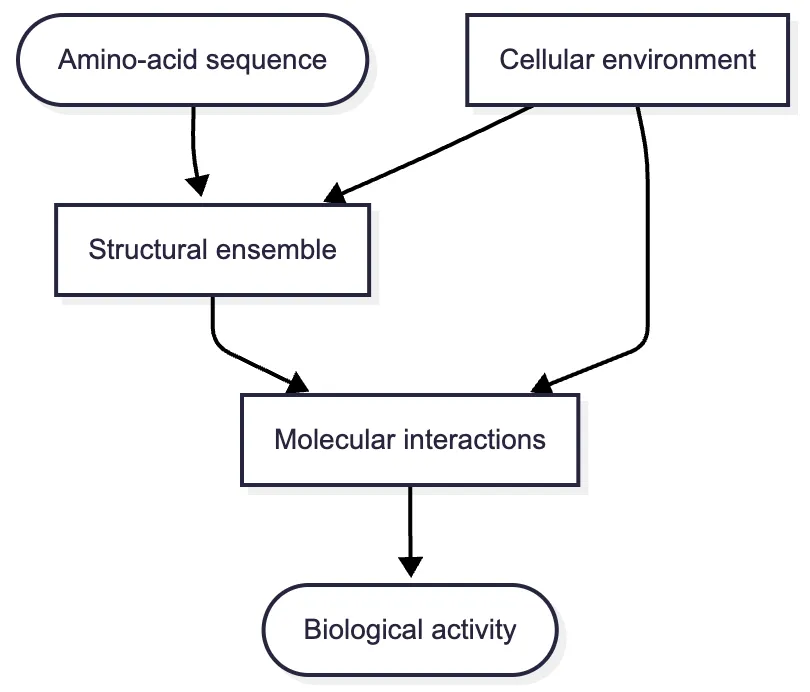
The diagram includes an ensemble rather than one structure. An ensemble is a collection of conformations with different probabilities. Many early computational methods sought a single representative structure because that was already difficult and because experimental databases were dominated by deposited coordinate sets. The later importance of dynamics does not make those static models useless; it clarifies what they approximate.

Why a structural archive changed the problem

Prediction requires examples against which ideas can be tested. X-ray crystallography, nuclear magnetic resonance spectroscopy, and later cryogenic electron microscopy made it possible to infer atomic coordinates experimentally. The Protein Data Bank (PDB), founded in 1971, turned those results into a shared, machine-readable archive.² Its importance was not simply that it stored pictures. Each entry connected a biological molecule, an experimental procedure, a sequence, and a set of coordinates. That made structural biology cumulative and eventually made supervised learning possible.

These techniques observe structure indirectly. Crystallography infers an electron-density pattern from how a crystal scatters X-rays; nuclear magnetic resonance uses signals from atomic nuclei to constrain distances and motions in solution; cryogenic electron microscopy reconstructs three-dimensional density from many images of rapidly frozen particles. Researchers then build atomic models into those measurements. A PDB coordinate is therefore an experimentally supported model with a resolution and uncertainty, not a literal photograph of stationary atoms.

The archive revealed a useful regularity: evolution often changes sequence more quickly than it changes the overall fold. Two proteins can descend from a common ancestor and retain similar structures despite many residue substitutions. Such proteins are homologues. If a query sequence resembles a protein with a known structure, the known structure can serve as a template. Chothia and Lesk quantified the relationship between sequence divergence and structural divergence, giving comparative modelling an empirical basis.³

Comparative, or homology, modelling then became a structured inference problem. One first identifies a template, aligns the query residues to the template residues, transfers corresponding geometrical restraints, builds unaligned loops and side chains, and refines the result. MODELLER formalized much of this process as the satisfaction of spatial restraints.⁴ Threading methods widened the search by asking whether a sequence was compatible with the residue environments of a known fold even when obvious sequence similarity had disappeared.⁵

These methods were powerful precisely because they did not solve folding from first principles. They exploited the fact that evolution repeatedly modifies existing proteins and that the archive already contained many reusable folds. Their limitation followed from the same source: when no suitable template existed, the search became much harder.

How physical search became practical enough to design with

Template-free methods approached the chain as a physical and statistical object. The Rosetta project, developed in David Baker’s group, began from an observation about local structure: short sequence fragments often adopt similar local conformations in known proteins. Rosetta assembled such fragments into candidate backbones and used a scoring function to favour globally coherent arrangements.⁶ Later versions used more detailed all-atom energy terms to represent packing, hydrogen bonding, electrostatics, and solvation.⁷

The key idea was not that fragment assembly reproduced the literal path by which a protein folds. It was a search strategy. Local fragments restricted the possibilities; the energy function ranked completed structures; repeated stochastic trials explored different combinations. The method exchanged an impossible exhaustive search for a guided but still expensive one.

Rosetta also made the reverse question approachable. If a backbone is specified, which sequence would make that structure energetically favourable? In 2003, Brian Kuhlman and colleagues reported Top7, a designed globular protein with a topology not previously observed in nature. Its experimental structure closely matched the computational model.⁸ The result mattered because it connected calculation to synthesis and structural measurement. The software had not merely recognized a naturally evolved fold; it had helped specify a new one.

Subsequent work distilled recurring geometric rules for “ideal” proteins, including preferred loop lengths and ways of packing helices and sheets.⁹ These rules reduced the search space and made design more systematic. They also exposed a theme that returns throughout this series: good generative methods do not sample every mathematically possible object. They encode constraints that make useful objects much more likely.

What the early programs actually computed

The names “comparative modelling” and “physical search” can obscure the computational objects these systems manipulated. At a high level, each program required four choices. It needed variables describing a candidate structure, a rule for proposing or calculating new values, a numerical objective for comparing candidates, and a search procedure for deciding which candidate to examine next. MODELLER and Rosetta shared this pattern but obtained their objectives and moves from different sources.

MODELLER began with an alignment between a query sequence and one or more template structures. Let $x$ denote the query's candidate coordinates, and let $g_r(x)$ be a geometric quantity—such as a distance, bond angle, or dihedral angle—measured from those coordinates. Corresponding template residues supplied a probability distribution $p_r$ for each quantity. Schematically, MODELLER minimized an objective of the form

The first sum penalizes geometries that the template-derived distributions consider unlikely; $w_r$ controls the influence of each restraint. The stereochemical term penalizes features such as distorted covalent geometry and overlapping atoms. A narrowly conserved template distance produces a sharp penalty when violated, whereas an uncertain alignment or variable loop can produce a broader restraint. The optimizer changes $x$ to reduce the total, so satisfying one restraint may require compromising with another. MODELLER therefore did not copy a template atom for atom. It converted uncertain structural correspondence into a joint optimization problem.⁴ This objective was useful for model construction, but it was not a complete physical free energy of the protein and solvent.

Rosetta represented the candidate primarily through backbone torsion angles. For each short sequence window—originally fragments of three and nine residues—it searched the structural database for fragments with compatible local sequences and predicted secondary structures. A trial move selected a window and replaced its current backbone angles with those from one library fragment. This proposal mechanism made the search discontinuous: instead of rotating every bond by a tiny amount, Rosetta could insert a locally protein-like arrangement in one step.⁶

After a move, Monte Carlo sampling compared the old and new scores. A standard acceptance rule can be written as

Any move that lowers the score is accepted. A move that raises it can still be accepted with a probability that becomes smaller as the score increase grows or as the computational temperature $T$ is lowered. Here, $T$ controls exploration; it need not equal the protein's physical temperature. Simulated annealing starts with greater tolerance for uphill moves and gradually becomes more selective. This prevents the search from being trapped immediately by the first locally favourable arrangement, but it cannot guarantee escape from every wrong basin. Thousands of independent trajectories were therefore useful because different random paths reached different structures.⁶⁷

Early Rosetta also separated two resolutions. A coarse “centroid” stage replaced each side chain with an approximate interaction centre, making large backbone moves inexpensive. Promising backbones then entered an all-atom stage, where side chains were assigned discrete conformations called rotamers and repacked. Its score had the schematic form ${\displaystyle S(x)=\sum _k{w}_k{E}_k(x),}$ where individual terms represented steric repulsion, hydrogen bonding, electrostatics, solvation, torsional preferences, and statistical patterns learned from known structures. The weights $w_k$ balanced quantities with different scales; the resulting score was an engineered ranking function rather than one exact experimentally measured energy.⁷ This division addressed a conflict that persists in generative modelling: broad exploration is easier with a simplified representation, while final discrimination requires chemical detail.

The implementation exposes two distinct failure modes. A sampling failure occurs when the search never proposes a near-native structure. A scoring failure occurs when such a structure is proposed but the objective ranks another candidate more favourably. More trajectories can reduce the first problem, but not the second. If an incorrect compact structure exploits a weakness in the score, more sampling can make that wrong minimum easier to discover. Search and scoring were therefore coupled in operation but remained separate scientific bottlenecks.

How neural networks entered before end-to-end folding

Machine learning was part of protein prediction decades before AlphaFold. The early target was usually secondary structure: local backbone patterns such as alpha helices, beta strands, and irregular coil regions. Predicting these categories is easier than placing every atom, but it tests whether a model can infer structural tendencies from sequence context.

In 1988, Ning Qian and Terrence Sejnowski trained neural networks to predict secondary structure from local sequence windows.¹⁰ The networks were small by modern standards and had no direct representation of global three-dimensional geometry. Their importance lay in demonstrating that nonlinear learners could recognize recurring sequence–structure relationships from examples.

PSIPRED later made a large practical improvement by supplying a neural network with position-specific profiles derived from related sequences.¹¹ Each profile summarized which amino acids appeared at one aligned position and how strongly they were conserved. The combination anticipated the next era: evolutionary preprocessing produced an informative representation, and a learned model converted it into structural predictions.

At the implementation level, PSIPRED first used PSI-BLAST to search a sequence database iteratively for relatives. The final search profile was a position-specific scoring matrix $X\in {ℝ}^{L\times 20},$ with one row for each of the $L$ query positions and one column for each standard amino acid. Conceptually, an entry can be read as a log-odds score, ${\displaystyle X_{ia}\approx \log \frac{p_i(a)}{p_{\mathrm{b}\mathrm{g}}(a)},}$ where $p_i(a)$ describes how compatible amino acid $a$ is with position $i$ among the detected relatives, and $p_{\mathrm{b}\mathrm{g}}(a)$ is its background frequency. A positive value therefore indicates that $a$ is more compatible with that family position than background expectation; a negative value indicates depletion. This row is richer than the identity of the query residue alone: it summarizes which substitutions evolution appears to have tolerated at that position. The original implementation mapped each score into the interval from zero to one using

To predict the class of residue $i,$ the first network flattened a 15-position window, from $i-7$ to $i+7,$ into one input vector ${𝐱}_i.$ The architecture can be written schematically as

Here, $H,E,$ and $C$ denote helix, strand, and coil; ${𝐨}_i$ contains their three output scores rather than atomic coordinates. The same learned weights were reused as the window slid along the sequence. In the original system, the window contributed $15\times 20$ profile values plus one chain-boundary indicator for each position, giving 315 inputs, followed by one hidden layer and three output units. During training, back-propagation adjusted the weights so that the output corresponding to the experimentally assigned secondary structure became more favourable. The network could consequently learn combinations of profile features rather than rely on a fixed rule such as “alanine favours helices.”¹¹

A second network then read the three first-stage scores across another 15-position window and produced revised $H/E/C$ scores. This was not merely cosmetic smoothing: it let the model learn that secondary-structure states usually persist for several residues and that, for example, an isolated one-residue helix is unlikely. Because each second-stage input already summarized a 15-position profile window, the final decision could indirectly depend on a span of up to 29 sequence positions. It still could not directly compare arbitrary distant residue pairs, represent how two chain segments pack, or generate three-dimensional coordinates. PSIPRED therefore illustrates both the strength and the boundary of pre-end-to-end learning: evolutionary information answered which residues fit each family position, while a neural network translated nearby patterns in that information into local structural labels.

How blind evaluation changed scientific progress

A prediction method can appear successful if it is tested on structures that influenced its design, if easy examples dominate the benchmark, or if failures remain unpublished. The Critical Assessment of protein Structure Prediction (CASP), initiated by John Moult and colleagues in 1994, addressed these problems with a recurring blind experiment. Organizers obtained sequences whose experimental structures were not yet public; modelling groups submitted predictions; and independent assessors compared predictions with the subsequently released structures.¹²

CASP gave the community more than a leaderboard. It separated template-rich from template-poor targets, made improvements visible under common conditions, and forced researchers to confront generalization. The competition also generated a history of changing bottlenecks. Better template detection and fragment assembly improved some categories; evolutionary information later transformed difficult targets; deep learning then altered the entire prediction pipeline.

Blind evaluation remains essential even though the data environment has changed. Today, a model may have seen billions of sequences, hundreds of millions of predicted structures, and many versions of the PDB. Excluding an identical test structure is no longer sufficient if close homologues, the same structural motif, or predictions derived from that target remain in training data. CASP’s durable contribution is the principle that evidence should be separated from the process that produced the model.

Conclusion

By the end of the 20th century, the field possessed the conceptual ingredients needed for machine learning: a sequence-to-structure premise, a growing archive of labelled examples, physical scoring functions, reusable structural templates, early neural networks for local secondary structure, and blind evaluation. What it still lacked was a way to infer long-range relationships reliably when no close template existed.

The next advance came from a source that had been present all along: evolution. A sequence database does not only contain many individual proteins. It contains the record of many related proteins changing together. Learning how to read that record turned sequence variation into approximate geometric information.

Onto the next article.

References

#Biology

References

Anfinsen, C. B. (1973). Principles that govern the folding of protein chains. Science, 181(4096), 223–230. https://doi.org/10.1126/science.181.4096.223↩
Berman, H. M., Westbrook, J., Feng, Z., Gilliland, G., Bhat, T. N., Weissig, H., et al. (2000). The Protein Data Bank. Nucleic Acids Research, 28(1), 235–242. https://doi.org/10.1093/nar/28.1.235↩
Chothia, C., & Lesk, A. M. (1986). The relation between the divergence of sequence and structure in proteins. The EMBO Journal, 5(4), 823–826. https://doi.org/10.1002/j.1460-2075.1986.tb04288.x↩
Šali, A., & Blundell, T. L. (1993). Comparative protein modelling by satisfaction of spatial restraints. Journal of Molecular Biology, 234(3), 779–815. https://doi.org/10.1006/jmbi.1993.1626↩
Bowie, J. U., Lüthy, R., & Eisenberg, D. (1991). A method to identify protein sequences that fold into a known three-dimensional structure. Science, 253(5016), 164–170. https://doi.org/10.1126/science.1853201↩
Simons, K. T., Kooperberg, C., Huang, E., & Baker, D. (1997). Assembly of protein tertiary structures from fragments with similar local sequences using simulated annealing and Bayesian scoring functions. Journal of Molecular Biology, 268(1), 209–225. https://doi.org/10.1006/jmbi.1997.0959↩
Rohl, C. A., Strauss, C. E. M., Misura, K. M. S., & Baker, D. (2004). Protein structure prediction using Rosetta. Methods in Enzymology, 383, 66–93. https://doi.org/10.1016/S0076-6879%2804%2983004-0↩
Kuhlman, B., Dantas, G., Ireton, G. C., Varani, G., Stoddard, B. L., & Baker, D. (2003). Design of a novel globular protein fold with atomic-level accuracy. Science, 302(5649), 1364–1368. https://doi.org/10.1126/science.1089427↩
Koga, N., Tatsumi-Koga, R., Liu, G., Xiao, R., Acton, T. B., Montelione, G. T., & Baker, D. (2012). Principles for designing ideal protein structures. Nature, 491(7423), 222–227. https://doi.org/10.1038/nature11600↩
Qian, N., & Sejnowski, T. J. (1988). Predicting the secondary structure of globular proteins using neural network models. Journal of Molecular Biology, 202(4), 865–884. https://doi.org/10.1016/0022-2836%2888%2990564-5↩
Jones, D. T. (1999). Protein secondary structure prediction based on position-specific scoring matrices. Journal of Molecular Biology, 292(2), 195–202. https://doi.org/10.1006/jmbi.1999.3091↩
Moult, J., Pedersen, J. T., Judson, R., & Fidelis, K. (1995). A large-scale experiment to assess protein structure prediction methods. Proteins: Structure, Function, and Genetics, 23(3), ii–iv. https://doi.org/10.1002/prot.340230303↩